Advection diffusion surface

In this notebook, we will solve the surface advection-diffusion equation using the finite element method (FEM) implemented in tatva. We will focus on 2D spherical surface embedded in 3D space.

The strong form of the surface advection-diffusion equation is given by:

\[ \frac{\partial c}{\partial t} + \nabla_s \cdot (\boldsymbol{u} c) - D \Delta_s c = f \quad \text{on } \Gamma \]

where $ c $ is the concentration of the substance on the surface $ \Gamma $, $ \boldsymbol{u} $ is the velocity field tangential to the surface, $ D $ is the diffusion coefficient. In this equation, $ \Delta_s $ is the Laplace-Beltrami operator on the surface, and $ f $ is a source term. Also, $ \nabla_S $ denotes the surface gradient which is given by projecting the standard gradient onto the tangent plane of the surface.

\[ \nabla_S = \mathbf{J}(\mathbf{J}^T\mathbf{J})^{-1} \nabla_\xi \]

where $\mathbf{J}$ is the Jacobian of the mapping from the reference element to the surface element.

Expanding the advection term using the product rule, we have:

\[ \nabla_s \cdot (\mathbf{u} c) = \boldsymbol{u} \cdot \nabla_s c + c \nabla_s \cdot \mathbf{u} \]

We assume that the velocity field $\boldsymbol{u}$ is divergence-free on the surface, i.e., $\nabla_s \cdot \boldsymbol{u} = 0$. This simplifies the advection term to:

\[ \nabla_s \cdot (\boldsymbol{u} c) = \boldsymbol{u} \cdot \nabla_s c \]

To derive the weak form, we multiply the equation by a test function $v$ and integrate over the surface $\Gamma$. Using integration by parts for the diffusion term, we obtain the weak form:

\[ \mathcal{W}(c, v) =\underbrace{\int_{\Gamma} \frac{\partial c}{\partial t} v ~ d\Gamma}_{\text{Inertia}} - \underbrace{\int_{\Gamma} c \boldsymbol{u} \cdot \nabla_s v ~ d\Gamma}_{\text{Advection (Conservative)}} + \underbrace{\int_{\Gamma} D \nabla_s c \cdot \nabla_s v ~ d\Gamma}_{\text{Diffusion}} - \underbrace{\int_{\Gamma} f v ~ d\Gamma}_{\text{Source}} \]

from typing import NamedTuple

import jax
import jax.numpy as jnp
import numpy as np
import pyvista as pv
from jax import Array
from jax_autovmap import autovmap
from tatva.utils import virtual_work_to_residual

from tatva import Mesh, Operator, compound, element, sparse

pv.set_jupyter_backend("client")
jax.config.update("jax_enable_x64", True)  # Use double-precision for FEM stability
jax.config.update("jax_platforms", "cpu")  # Change to "gpu" if available

We start with creating the mesh for the spherical surface of radius 1.0 using gmsh.

def create_sphere_mesh(r=1.0, lc=0.5):
    import gmsh

    gmsh.initialize()
    gmsh.model.add("Sphere")
    gmsh.model.occ.addSphere(0, 0, 0, r)
    gmsh.model.occ.synchronize()
    gmsh.option.setNumber("Mesh.MeshSizeMax", lc)
    gmsh.model.mesh.generate(2)  # Surface mesh only

    _, coords, _ = gmsh.model.mesh.getNodes()
    nodes = jnp.array(coords.reshape(-1, 3))

    _, _, node_indices = gmsh.model.mesh.getElements(2)
    elements = jnp.array(node_indices[0].reshape(-1, 3) - 1)

    gmsh.finalize()
    return Mesh(coords=nodes, elements=elements)


radius = 1.0
mesh = create_sphere_mesh(r=radius, lc=0.05)
n_dofs = mesh.coords.shape[0]

Info    : Meshing 1D...
Info    : [ 40%] Meshing curve 2 (Circle)
Info    : Done meshing 1D (Wall 0.000460455s, CPU 0s)
Info    : Meshing 2D...
Info    : Meshing surface 1 (Sphere, Frontal-Delaunay)
Info    : Done meshing 2D (Wall 0.425447s, CPU 0.419692s)
Info    : 6093 nodes 12247 elements

In order to the surface PDE, we define a triangular element (topology in 2D) embedded in 3D space. We then define the surface gradient operator using the Jacobian of the mapping from the reference element to the surface element. Finally, we assemble the mass and stiffness matrices using the surface gradient operator.

def safe_sqrt(x):
    return jnp.where(x < 0, 0.0, jnp.sqrt(x))


class Tri3Manifold(element.Tri3):
    """A 3-node linear triangular element on a 2D manifold embedded in 3D space."""

    def get_jacobian(self, xi: Array, nodal_coords: Array) -> tuple[Array, Array]:
        dNdr = self.shape_function_derivative(xi)
        J = dNdr @ nodal_coords  # shape (2, 2) or (2, 3)
        G = J @ J.T  # shape (2, 2)
        detJ = safe_sqrt(jnp.linalg.det(G))
        return J, detJ

    def gradient(self, xi: Array, nodal_values: Array, nodal_coords: Array) -> Array:
        dNdr = self.shape_function_derivative(xi)  # shape (2, 3)
        J, _ = self.get_jacobian(xi, nodal_coords)  # shape (2, 3)

        G_inv = jnp.linalg.inv(J @ J.T)  # shape (2, 2)
        J_plus = J.T @ G_inv  # shape (3, 2)

        dudxi = dNdr @ nodal_values  # shape (2, n_values)
        return (J_plus @ dudxi).T  # shape (3, n_values)

We can now use the custom-defined element Tri3Manifold and define an Operator.

tri3 = Tri3Manifold()
op = Operator(mesh, tri3)

To check if the implementation is correct, we compute the total surface area by integrating the constant function 1 over the surface. The total area should match the known analytical value for the given surface.

print(f"Calculated surface area {op.integrate(1.0)}")  # Warm-up
print(f"Actual surface area {4 * jnp.pi * radius**2}")

Calculated surface area 12.5600450452555
Actual surface area 12.566370614359172

We now compute the normals and also check if the normals are computed correctly by plotting them on the surface mesh. We use op.map function to map the get_jacobian function of our Tri3Manifold element to all the quadrature points of all elements. This will give us a new function to which we can give mesh coordinates and get Jacobians at all the quadrature points.

@autovmap(J=2)
def get_normals(J: Array) -> Array:
    """Computes the normal vector to the surface given the Jacobian J."""
    n = jnp.cross(J[0, :], J[1, :])
    n = n / jnp.linalg.norm(n)
    return n


J, _ = op.map(tri3.get_jacobian)(mesh.coords)
normals = get_normals(J)

Simulating the Advection-Diffusion equation¤

Now, we can start with defining the problem parameters and initial conditions. We will discretize the time domain and use the implicit Euler method for time integration.

class TransportPhysics(NamedTuple):
    epsilon: float = 0.05  # Diffusivity (Viscosity)
    dt: float = 0.01


transport_params = TransportPhysics()


@autovmap(coords=1)
def get_shear_velocity(coords):
    x, y, z = coords
    # Angular velocity varies with z (latitude)
    # e.g., Fast equator, stationary poles: omega = 5 * (1 - z^2)
    # e.g., Counter-rotating bands: omega = 5 * jnp.sin(3 * jnp.pi * z)
    omega = 10.0 * jnp.sin(3.0 * jnp.pi * z)

    # Cross product of (0,0,omega) and (x,y,z)
    u = jnp.array([-y * omega, x * omega, 0.0])
    return u


@autovmap(coords=1)
def get_deformational_velocity(coords):
    """
    Computes a divergence-free deformational flow.
    Stream function psi = x * y * z
    u = curl(psi * x_vec) = grad(psi) x x_vec
    """
    x, y, z = coords
    magnitude = 20.0  # Adjust speed

    u_x = x * (z**2 - y**2)
    u_y = y * (x**2 - z**2)
    u_z = z * (y**2 - x**2)

    return magnitude * jnp.array([u_x, u_y, u_z])


nodal_velocity = get_deformational_velocity(mesh.coords)
# nodal_velocity = mesh.coords @ jnp.array([[0.0, 1.0, 0.0],[-1.0, 0.0, 0.0], [0.0, 0.0, 0.0]])

# Precompute velocity at quadrature points
u_quad = op.eval(nodal_velocity)

Code for velocity visualization using PyVista

faces = np.column_stack(
    [np.full(len(mesh.elements), 3, dtype=np.int64), mesh.elements.astype(np.int64)]
).flatten()

surf = pv.PolyData(np.array(mesh.coords), faces)
surf.point_data["v"] = nodal_velocity
surf.set_active_vectors("v")

pl = pv.Plotter()
pl.add_mesh(surf, color="lightgray")
pl.add_arrows(mesh.coords, nodal_velocity, mag=0.015, color="#009AF9")
pl.view_isometric()

Velocity field

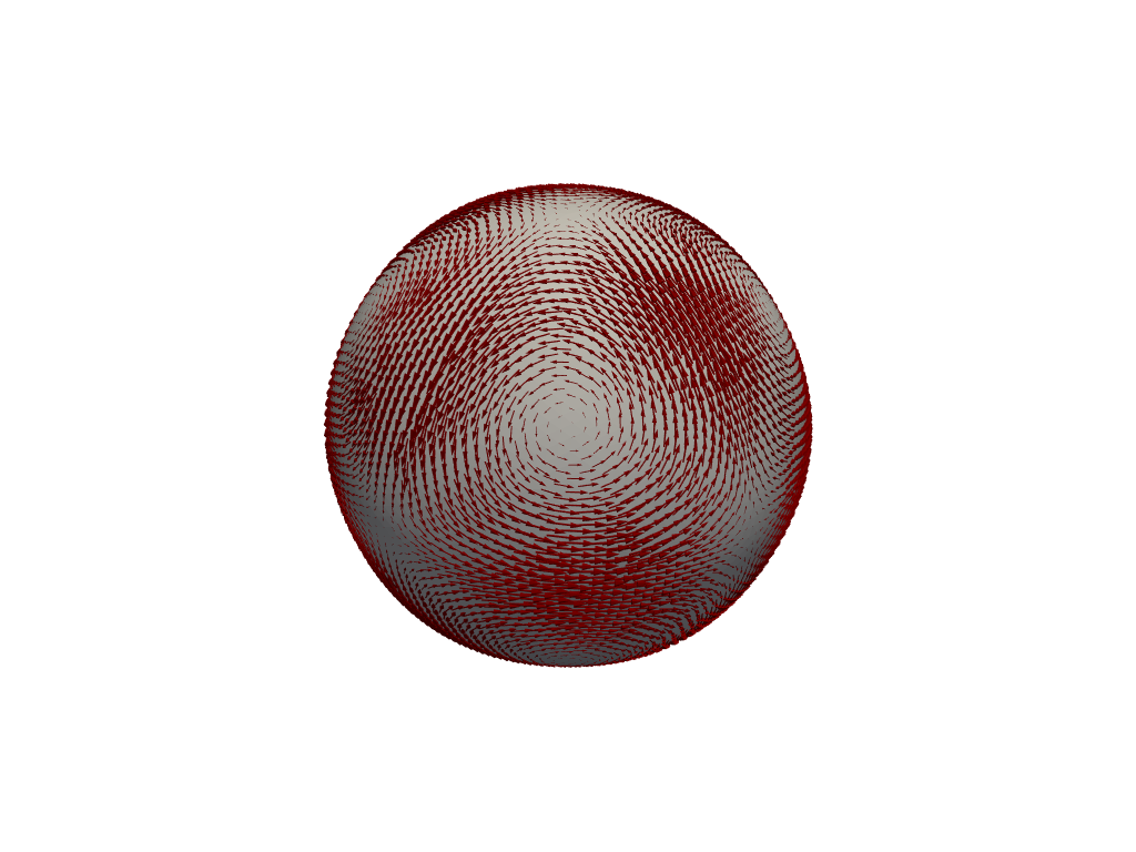
Now we define functions to compute the total virtual work and total kinetic energy.

The very first thing we define is our concentration field using the tatva.compound.Compound. This class basicaly initially a jax array of correct shape and siye based on the mesh that we pass since we passed compound.FieldSiye.AUTO as first argument of the shape tuple and since concentration is scalar we dont define the second argument of the shape tuple. We also define the field_type to be nodal values.

class Concentration(compound.Compound, mesh=mesh):
    c = compound.field(
        shape=(compound.FieldSize.AUTO,), field_type=compound.FieldType.NODAL
    )

Creating non-variational form¤

To create a non-variational form, we define a function that takes both trial and test function and then we create our integrand using these two variable.

@autovmap(grad_c=1, v=0, grad_v=1, u_quad=1, epsilon=0)
def compute_advection_diffusion_density(grad_c, v, grad_v, u_quad, epsilon):
    """
    Computes the virtual work density for Advection-Diffusion.

    Args:
        c, v: Scalar values of trial and test functions
        grad_c, grad_v: Surface gradients
        u_quad: Velocity vector at quad point
        epsilon: Diffusivity
    """
    term_diffusion = epsilon * jnp.vdot(grad_c, grad_v)

    advection_flux = jnp.vdot(u_quad, grad_c)
    term_advection = advection_flux * v

    return term_diffusion + term_advection


@autovmap(c=0, v=0)
def compute_kinetic_energy_density(c: Array, v: Array) -> Array:
    """Computes the kinetic energy density: 0.5 * c * v
    Args:
        c, v: Scalar values of trial and test functions
    """

    return jnp.dot(c, v)


@jax.jit
def total_virtual_work(
    v_flat: Array, c_flat: Array, c_old_flat: Array, dt: float
) -> Array:
    """
    Computes the spatial part of the weak form: Integral(Advection + Diffusion)
    Args:
        v_flat: Flattened nodal values of test function
        c_flat: Flattened nodal values of trial function
        c_old_flat: Flattened nodal values of trial function at previous time step
        dt: Time step size
    """

    (c,) = Concentration(c_flat)
    (v,) = Concentration(v_flat)
    (c_old,) = Concentration(c_old_flat)

    c_quad = op.eval(c)
    v_quad = op.eval(v)
    c_old_quad = op.eval(c_old)

    grad_c = op.grad(c)
    grad_v = op.grad(v)

    # compute density
    density = compute_advection_diffusion_density(
        grad_c, v_quad, grad_v, u_quad, transport_params.epsilon
    )

    # compute kinetic energy density
    kinetic_energy_density = (
        compute_kinetic_energy_density(c_quad - c_old_quad, v_quad) / dt
    )

    # compute total energy
    total_energy = op.integrate(density + kinetic_energy_density)

    # integrate over the surface
    return total_energy

tatva provides a helper function to convert this virtual work to resdiual by taking the deriavtive with respect to test function and setting it to 0 i.e

\[ \boldsymbol{r} = \frac{\partial \mathcal{W}(u, v)}{\partial v}\Big|_{v=0} \]

We define the residual function using virtual_work_to_residual, which converts the total virtual work function into a residual function. We use sparse differentiation to compute the Jacobian of the residual function. The sparisty pattern needed is automatically computed from the virtual work function. To get the sparsity pattern of a virtual form, we use the functionality tatva.sparse.pattern_from_virtual_work.

compute_residual = virtual_work_to_residual(
    total_virtual_work, test_size=Concentration.size, jit=True
)

sparsity_pattern = sparse.pattern_from_virtual_work(
    total_virtual_work,
    Concentration.size,
    "c_flat",
    "v_flat",
    jnp.zeros(Concentration.size),
    1.0,
)
cm = sparse.ColoredMatrix.from_csr(sparsity_pattern)
n_colors = int(cm.colors.max() + 1)
print(f"Number of colors: {n_colors}")

hessian_fn = sparse.jacfwd(
    compute_residual, colored_matrix=cm, color_batch_size=n_colors
)
hessian_fn = jax.jit(hessian_fn)

Number of colors: 14

Initial Condition¤

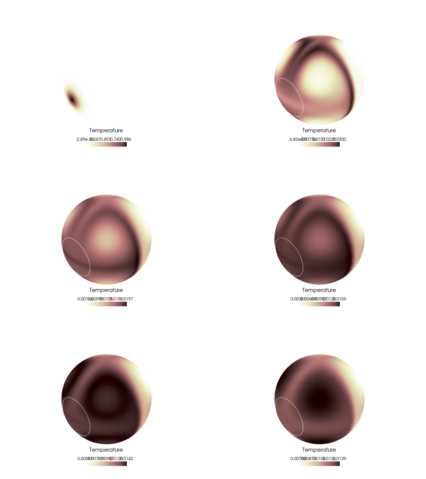
Initially, we set the concentration field to be a Gaussian distribution centered at a specific point on the surface. We also define a tangential velocity field that will advect the concentration over time. Finally, we run the time-stepping loop to solve the advection-diffusion equation on the surface. We visualize the concentration field at each time step to observe how it evolves over time.

# Initial Condition: Gaussian Blob
def get_gaussian_initial_condition(
    mesh_coords, pole=jnp.array([0.0, 0.0, 1.0]), sigma=0.2
):
    # Calculate squared Euclidean distance from each node to the pole
    # distances: (n_nodes,)
    dists_sq = jnp.sum((mesh_coords - pole) ** 2, axis=1)

    # Gaussian distribution
    u_0 = jnp.exp(-dists_sq / (2 * sigma**2))
    return u_0


def compute_total_concentration(c_flat):
    (c,) = Concentration(c_flat)
    return op.integrate(c)

Transient solve¤

    mesh.coords, pole=jnp.array([1, 0.0, 0.0]), sigma=0.15
)

c_history = [c_curr]
total_conc_per_time = [compute_total_concentration(c_curr)]

n_steps_transport = 100
dt_transport = 0.05

for step in range(n_steps_transport):
    rhs = -compute_residual(c_curr, c_curr, dt_transport)

    A = hessian_fn(c_curr, c_curr, dt_transport)

    delta_c = jax.experimental.sparse.linalg.spsolve(A.data, A.indices, A.indptr, rhs)

    c_curr = c_curr + delta_c
    c_history.append(c_curr)

    total_conc = compute_total_concentration(c_curr)
    total_conc_per_time.append(total_conc)

    if step % 10 == 0:
        print(f"Step {step}: Max c = {jnp.max(c_curr):.4f}")

Output

Step 0: Max c = 0.7171 Step 10: Max c = 0.0269 Step 20: Max c = 0.0188 Step 30: Max c = 0.0153 Step 40: Max c = 0.0141 Step 50: Max c = 0.0139 Step 60: Max c = 0.0137 Step 70: Max c = 0.0133 Step 80: Max c = 0.0130 Step 90: Max c = 0.0127

Visualization of the concentration evolution¤

Post-processing and Visualization

sargs = dict(
    title=r"Concentration" + "\n",
    height=0.08,  # Reduces the length (25% of window height)
    width=0.2,  # Adjusts thickness
    vertical=False,  # Orientation
    position_x=0.4,  # Distance from left edge (5%)
    position_y=0.08,  # Distance from bottom edge (5%)
    title_font_size=20,
    label_font_size=16,
    color="black",  # Useful for white/transparent backgrounds
    font_family="arial",
)
pv.set_jupyter_backend("server")
surf = pv.PolyData(np.array(mesh.coords), faces)
surf.point_data["c"] = c_history[10].flatten()
surf.point_data["v"] = nodal_velocity
surf.set_active_scalars("c")

contours = surf.contour(isosurfaces=10)

pl = pv.Plotter()
pl.add_mesh(surf, scalars="c", cmap="pink_r", scalar_bar_args=sargs)
pl.add_mesh(contours, cmap="pink_r", line_width=0.5, show_scalar_bar=False)
pl.show()

Widget(value='<iframe src="http://localhost:46633/index.html?ui=P_0x7d49510aee90_6&reconnect=auto" class="pyvi…

Concentration evolution on spherical manifold